Grit Behavior In Splitting Structures: Model-To-Prototype Confidence

By Stuart Cain

Using computational fluid dynamics, engineers can all but guarantee their design solution for an all-too-common wastewater influent issue.

Wastewater treatment plants are hydraulically designed to handle a wide range of inflows and grit loads. Wastewater and grit flow into the plants from sewers connected to municipal homes and businesses as well as runoff from impermeable surfaces. The influent initially passes through a screening facility designed to remove large pieces of trash and floatables. Sewage pumps are then typically used to lift the wastewater from the screening chamber to the primary treatment level of the plant. The first stage of primary treatment is commonly a series of primary settling tanks, arranged in parallel, designed to promote sedimentation by slowing the treatment flow and allowing gravity to remove grit.

Before water enters the primary settling tanks, a flow-splitting structure is commonly required to promote equal flow and equal grit split between the tanks. Equal flow and equal grit distribution between operating settling tanks is necessary to optimize the performance of the primary treatment systems. As part of the design process, hydraulic modeling of the flow-splitting structure is typically performed to assure equal distribution of flow of water and grit to each tank, with the goal of obtaining a variation of flow and grit between tanks of no more than +/- 5 to 10 percent.

Historically, scaled physical modeling was performed to demonstrate required splitting structure performance, and well-known scaling laws provided assurance of good model-to-prototype correlation. More recently, three-dimensional numeric modeling (computational fluid dynamics [CFD]) is being used by designers to model these systems. Selecting the correct modeling approach and parameters is critical for assuring agreement between the model and the prototype performance.

CFD Modeling Of Flow-Splitting Structures

CFD modeling can be a powerful tool for optimizing the design of flow-splitting structures. However, model-to-prototype performance can be assured only if the appropriate numeric approach is taken to simulate the interactions between the flow, grit, and physical structure. Modeling assumptions are also critical, as is the selection of the modeling parameters. There are multiple approaches to treating the grit particles in a given CFD simulation, and selecting the inappropriate approach can result in significant deviation in simulated grit trajectories and settlement characteristics from that observed in the prototype system.

To demonstrate the numeric modeling process, an example of a flow-splitting structure design using CFD simulation is presented and selection of key modeling parameters highlighted.

Case Study: CFD Simulation Of A Flow-Splitting Structure

The purpose of this example design project was to develop a new flow-splitting structure (FSS) to distribute flow and grit uniformly to a series of four to five primary settling tanks (PSTs). The objectives of the associated CFD modeling effort were to:

• Determine the flow and grit distribution to the PSTs in the FSS under different operating conditions.
• Predict the water surface elevation in the inflow chamber and upstream of the overflow weirs in the FSS.
• Suggest modifications to optimize hydraulic and sedimentation performance in the FSS and evaluate the modified FSS designs to select the most robust final design.
• Minimize settling of grit in the FSS and related piping under various flow conditions.

The effort began with a base design and evolved through several design iterations (based on analyses of several CFD simulation results) before a final prototype design was selected.

Model Geometry and Flow Conditions

The general FSS geometry of the final, selected design is shown in Figure 1. In this example, there are two 78” diameter inlet pipes; one is in operation, and the other reserved for future flow conditions. The pipe in operation includes a vertical section, immediately followed by a 90° turn, a 45° horizontal turn, and a straight segment leading to the inflow chamber. There are two 36” diameter straight horizontal inlet pipes. One 36” pipe is in operation, and the other is idle. An inflow chamber connects the inlet pipes to the FSS. The FSS includes a 45° conduit immediately followed by a vertical conduit and an expansion to four (4) separate vertical chambers. The chamber at each side leads flow to two (2) separate control weirs. The two (2) chambers in the middle each pass flow to four (4) separated weirs (two on each side). A collection channel collects flow from the two weirs at opposite sides and passes flow to a compartment, which then feeds the PST. Conduits to each PST include five diameters of linear length to facilitate specification of outflow boundary conditions.

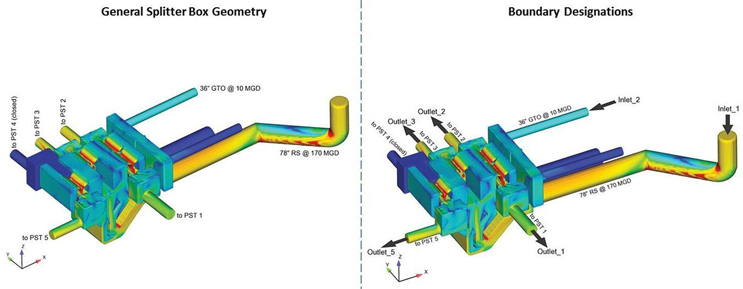
Figure 1. Splitter box geometry and boundary specification

Three design flows were considered in the simulation process:

• 35 MGD (25 MGD from one 78” RS pipe, 10 MGD from the 36” GTO pipe) with five (5) PSTs online,
• 180 MGD (170 MGD from one 78” RS pipe, 10 MGD from the 36” GTO pipe) with four (4) PSTs online, and
• 245 MGD (115 MGD from each of the two 78” RS pipes, 15 MGD from one 36” GTO pipe) with five (5) PSTs online.

General Model Description

The commercial CFD code FLOW-3D by Flow Science was used to perform the three-dimensional numeric simulations. FLOW-3D uses the Fractional Area/Volume Obstacle Representation (FAVOR) method for the modeling of solid obstacles, such as topology and structural members, allowing complex shapes to be simulated without resorting to stair-stepping the boundaries. The location of the free water surface is computed using the Volume of Fluid (VOF) method. This formulation consists of a scheme to describe the shape and location of the free surface, a method to track the evolution of the shape and location of the free surface through time and space, and a means for applying boundary conditions to the free surface.

An important objective of the modeling is to reliably predict the grit distribution in the FSS and, ultimately, the volume transported to each PST. There is an interaction between the turbulent flow and grit that is carried by the flow which requires a more complicated and robust model to predict the movement of grit. A state-of-the-art sediment scour model is required for this purpose.

The grit scour model in FLOW-3D was used to predict the erosion and deposition of grit. The model calculates the grit flux due to entrainment from the packed-bed interface and the drifting and deposition by computing the advection of the grit suspended in the flow, the settling of grit due to gravity, the resuspension (entrainment) of the grit due to shearing and flow turbulence, and the bed load transport (rolling, hopping, sliding along the packed bed). The grit can be at only two states: in suspension or packed. Suspended grit advects with fluid flow. Packed grit exists in the computational domain at a predefined critical packing fraction. There is only a thin layer of the packed grit that can move in the form of bed load transport. The calculation of grit was coupled with the fluid dynamics. The grit scour model is suitable for deposition and entrainment of sand, silt, and other non-cohesive sediment-type particles.

A few key assumptions were important to set grit modeling parameters and accurately simulate the grit transport — and deposition — process:

• The grit is non-cohesive.
• The grit is spherical in shape.
• The maximum packing fraction was 0.64. Hence, in each computational cell, the deposition of sediment stopped once the accumulated volume fraction of the sediment reached 64 percent of the cell volume.
• In the calculation of the drift velocity, a drag function combines the form drag and Stokes drag. Using this combined drag force to compute the momentum exchange between two particles is not quite correct. A commonly used approach is the Richardson-Zaki correction, which accounts for particle-particle interactions based on an experimentally determined relation. The Richardson-Zaki coefficient multiplier was 1.0, which means that the enhancement to the drag due to particle-particle interaction is exactly as defined by the Richardson-Zaki model.
• The critical Shields number is the dimensionless critical shear. The critical shear stress of a particle is defined as the minimum boundary shear stress necessary to initiate motion. For this example, the critical shear stress to move sewer deposits is taken from the recommended values from a few researchers based on an extensive literature review.
• The entrainment coefficient in the equation of sediment entrainment lift velocity is used to control the rate of sediment erosion at a local shear stress greater than the critical shear stress. This coefficient can be used to scale the scour rate or to fit the experimental data.
• The bed load coefficient in the Meyer-Peter and Mueller equation is used to control the rate at which bed load transport occurs at a local shear stress greater than the critical shear stress.
• The angle of repose of sediment is the maximum resting angle of the sediment bed and is used to modify the local critical Shields parameter. The repose angle was set to 30°.

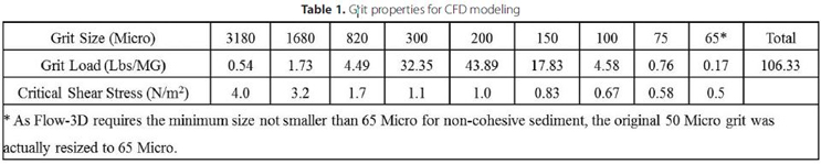
Table 1. Grit properties for CFD modeling

Boundary Conditions

Model inflow and outflow boundaries are shown in Figure 1. At the inlets, the volume flow rate was specified. At the outlets (leading to each PST), a pressure boundary condition (zero stagnation pressure and fluid elevation) was specified. Turbulence quantities also require specification at the model inlets, including turbulent kinetic energy and its dissipation rate.

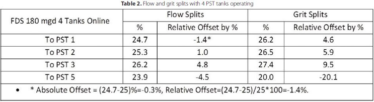
Table 2. Flow and grit splits with 4 PST tanks operating

Another important input at the inlets is the properties of the grit. For this example study, the grit size distribution and loading are listed in Table 1. The specific density of the modeled grit is 2.65. The critical shear stress for each grit size is also listed.

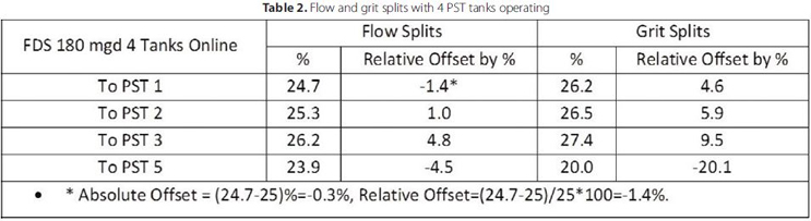
Table 3. Flow and grit splits with 5 PST tanks operating

Results

Several iterations of the FSS design were investigated as shown in Figure 2. Each design was evaluated for flow split, grit split, and grit settling within the FSS. The final design selected is shown in Figure 3 along with selected velocity, water level, and grit settling results. Flow and grit splits for the final design with four PST tanks operating are shown in Table 2. For the four PST operations considered, an even split between outflow conduits is 25 percent. The flow distribution is very close to an even split with maximum absolute offset of less than 2 percent and relative offset of less than 5 percent, with slightly more flow favored to PST 3. The grit distribution is not as uniform as the flow distribution. The maximum absolute grit distribution differs from the even value by about 5 percent, and the maximum relative offset is 20 percent. Slightly more grit favored PST 3 and less grit went to PST 5.

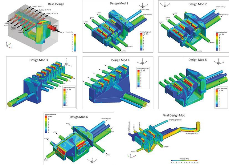
Figure 2. Evolution of splitter box design

Flow and grit splits are listed in Table 3 for five PST tanks operating. Flow distribution is very close to an even split (20 percent each) with maximum absolute offsets less than 1 percent and relative offsets less than 4 percent. Grit distribution is not as good as flow distribution, although it follows the general trend. The maximum absolute grit distribution is off the even distribution by about 4 percent, and the relative offset is 16.9 percent. Slightly more grit favored PST 2 and less grit passes to PST 5.

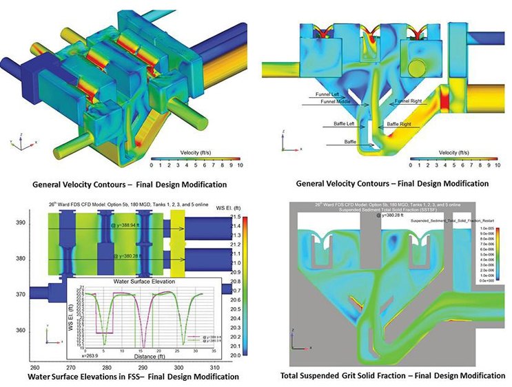
Figure 3. Selected results - final splitter box design

Confidence in the scale-up of the hydraulic performance of splitting structures is dependent upon the accuracy of the modeling conducted during the design process. With increased use of numeric models, particular attention must be paid to the numeric modeling approach chosen, the modeling assumptions, and the modeling parameters specified. Prior to using CFD modeling in a complex design effort such as flow splitter structures, validation against physical modeling and/or field test data should be conducted. A robust, scalable design can be developed using CFD modeling tools, and confidence in prototype performance can be realized, if experienced modelers are engaged in the design process.

---

About The Author

Stuart Cain, Ph.D., is the president of Alden Research Laboratory. He joined the company in 1996 to establish the Numeric Modeling Group and has over 25 years of experience in CFD modeling of complex water flow processes, including chemically reacting flows and particulate transport. As part of his technical responsibilities at Alden, he oversees projects involving both physical and CFD modeling of hydraulic processes in water treatment, distribution, and storage systems.