The $1.5 Million Sewer Repair — And The Water-Quality Evidence Missing Upstream

By Alex Towfigh

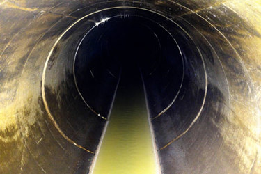
A California wire manufacturer was ordered to pay $1.5 million in restitution after acidic wastewater from its operations damaged a public sewer line. In its 2010 announcement, the U.S. EPA described 14 illegal discharges recorded during four months of 2008, with pH readings as low as 1 — far below the discharge permit’s minimum pH of 6.¹ The unsettling feature of this case is not one dramatic sensor reading. It is the opportunity for recurring chemical excursions to become a costly infrastructure failure before their source and pattern are resolved.

The investigation began when a sanitation-district employee encountered water around pH 3 in the Irwindale Trunk Line. Investigators traced the flow to Davis Wire, a galvanized-wire manufacturer whose process used sulfuric acid and was required to neutralize wastewater before discharge. The EPA stated that the facility’s treatment system had needed upgrades for years.¹

The restitution addressed cumulative sewer damage; it was not the price of a single slug and is not evidence that a new analyzer alone could have stopped the discharges. Proper neutralization equipment, maintenance, and permit compliance remained fundamental. The additional intelligence question is narrower: could a plant have recognized a developing, repeated failure pattern early enough to investigate a malfunctioning or bypassed treatment process?

THE COSTLY PATTERN: A recurring off-normal discharge can accumulate infrastructure consequences long before it becomes a familiar alarm pattern.

The case exposes a distinction between measuring a permitted endpoint and explaining a failure mechanism. A pH instrument at the discharge point can detect whether neutralization is producing an acceptable result. It does not, by itself, reveal whether an upstream transfer, failed dosing sequence, bypass, depleted reagent supply, or maintenance condition caused repeated off-spec water. Nor does a downstream sample necessarily retain the timing needed to reconstruct the originating plant event.

Better detection cannot replace functioning treatment equipment. It can, however, shorten the distance between a suspect reading and the evidence needed to fix the cause. That requires the exact sample point and timestamp, flow and pump state, neutralization history, instrument-health checks, and a traceable operating sequence. A system that merely adds another red icon to the control room offers less than one that produces a testable explanation of the recurring event.

The question worth taking to the next operations meeting

For each recurring discharge, identify (1) the earliest validated water-quality measurement, (2) the upstream equipment and process records needed to explain it, and (3) the authorized operating change capable of preventing its recurrence. If only the last downstream alarm is visible, the facility may know that a limit was crossed without knowing what to correct.

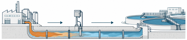
Figure 1. Conceptual source-to-treatment pathway. Upstream monitoring creates a possible intervention window; the illustration does not depict the actual Irwindale infrastructure.

There Are Two Bills For The Same Discharge

The receiving utility sees the environmental and infrastructure bill: corrosion, treatment instability, sampling, investigation, temporary chemical changes, or biological-process recovery. The manufacturer may be carrying another cost entirely: valuable product discharged during changeovers, avoidable wash-water loading, excess neutralization chemistry, or lost production hours. The two exposures are related, but they cannot automatically be added together as if each dollar were recoverable.

The industrial-product side is frequently absent from a wastewater calculation. Published dairy-process research, for example, estimated nonaccidental milk and dairy product losses to sewer at 1%–3% of total milk processed, particularly during starts, stops and rinse transitions.² Those percentages are evidence for the studied dairy context, not for food manufacturing or industry at large.

Consider what that published range implies at the scale of a documented four-million-pound-per-day dairy facility.³ At the USDA’s October 2026 all-milk price forecast of $19.90 per hundredweight, 1%–3% corresponds to approximately $7,960–$23,880 of raw-milk-equivalent value per operating day — or $2.39 million–$7.16 million over 300 operating days.⁴ These are arithmetic scenarios, not measured losses at that facility, not recoverable margin, and not a prediction of recoverable savings. Even if a fraction of the material is technically recoverable, it has to be identified separately from the wastewater-treatment charges it creates.

MATERIAL AND TREATMENT ARE SEPARATE LEDGERS: A lost product stream may have economic value upstream and create added wastewater load downstream. Avoid counting the same avoided cost twice.

The Treatment Bill Can Be Modeled From A Single Measured Parameter

Some municipalities calculate commercial and industrial sewer charges using flow and strength. San Diego’s published January 2026 commercial/industrial rates include $0.27 per pound of chemical oxygen demand (COD), $0.68 per pound of total suspended solids (TSS), and $3.85 per hundred cubic feet of wastewater flow. Facility-specific measured strengths can replace industry estimates.⁵

Suppose a site discharges one million gallons per operating day and a recurring process event adds 1,000 mg/L of COD to the wastewater above an otherwise comparable baseline. The mass increment is 1.0 million gal/day × 1,000 mg/L × 8.34 / 1,000,000 = 8,340 pounds COD per day. At $0.27 per pound, the modeled COD component alone is $2,252 per day, or approximately $675,500 over 300 days. Doubling the incremental concentration to 2,000 mg/L doubles that illustrative rate component to about $1.35 million annually.

This is a sensitivity calculation using a published local rate — not a billing forecast. It assumes the extra load is chargeable under the applicable measurement and billing arrangement for 300 days, and excludes flow, TSS, base fees, discharge permits, minimums, rate adjustments, and any recovery or treatment expense. The example also says nothing about how much of the COD represents saleable material. The value emerges only when concentration is connected to flow, timing, and the process that produced it.

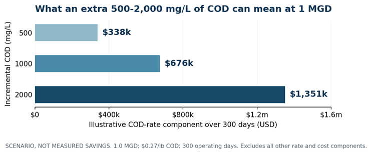
Figure 2. Illustrative COD-rate exposure at a stated flow and local published unit rate. These amounts are not measured plant losses, guaranteed billing changes, or projected AquaMesh savings.

The Expensive Blind Spot Is Usually Between Systems

Why connecting evidence is harder than adding another monitor

A useful investigation starts with records the facility already owns. Read-only access to PLC, SCADA, and historian tags — using appropriate interfaces such as OPC UA, Modbus, or MQTT where available — reconstructs production state, valve and pump events, operator interventions, instrument status and treatment conditions. Timestamps must be aligned and checked against actual hydraulic residence time. None of this requires placing an outside analytics system in charge of interlocks or dosing.

The remaining gap is often a physical measurement, not another trend display. A multiwavelength UV/visible optical sensor observes the spectral response of water across wavelengths; under suitable, site-calibrated conditions that fingerprint may flag a change in dissolved or suspended material that a single pH, flow, or conductivity tag cannot explain. It does not automatically identify a substance or measure every constituent. Matrix interference, bubbles, fouling, drift, and laboratory correlation determine whether the added signal is decision-grade.

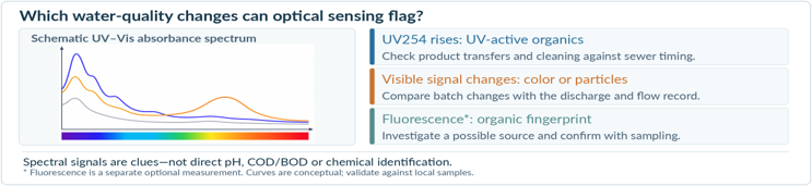
Spectral sidebar (schematic). UV-active organics, color, and suspended-material changes can be useful clues; spectral readings must be interpreted against flow, process timing, and laboratory results.

A process-aware model can align that physical change with a transfer, rinse, batch sequence, or industrial discharge, then ask whether sensor cleaning, temperature, upstream source-water quality, or travel-time differences provide a simpler explanation. Only after testing alternatives should it estimate downstream loading or the likely time remaining before a treatment unit is affected. The output is a documented, reviewable hypothesis and a targeted next check — not an autonomous instruction to override existing controls.

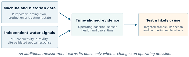
Figure 3. Technical evidence chain: existing machine records and independent water measurements are aligned by event timing, then used to test competing explanations. Conceptual architecture; performance depends on site validation.

An industrial historian can confirm that a transfer pump ran, a valve switched and a rinse began. It cannot reveal the composition of material in a pipe if no suitable instrument measures it. Flow establishes how much water moved; conductivity describes the combined ionic response; pH measures acid–base condition; laboratory analysis can identify constituents, often after a transient has passed. A new dashboard that simply plots those signals alongside one another leaves the physical blind spot untouched.

Consider a hypothetical ingredient line that finishes transfer at 14:03, begins a rinse at 14:06 and produces a change in wastewater optical response at 14:11. The first task is to reconcile clocks and the travel time from equipment to sensor. The second is to compare the event against matched production sequences: Was the change normal first-rinse carryover, a poorly seated valve, an altered recipe, an interfering cleaning chemical, or a dirty optical window? The third is to check an independent grab sample and, where appropriate, an upstream mass balance. A correlation between the rinse and the downstream signal is a lead — not a product-loss finding.

This is the use case for composition-sensitive sensing. UV/visible spectral measurements can provide a continuously sampled fingerprint that may respond to changes in the water matrix even when a conventional scalar tag is within limits. The signal is not a universal chemical identification and cannot replace laboratory COD, BOD, or regulatory analysis. Near-infrared, Raman, fluorescence, or targeted process analyzers may be better for some constituents. The engineering choice is the least additional measurement that materially changes a decision, not the most elaborate sensor. The Water Research literature emphasizes calibration as fundamental to quantitative UV/Vis interpretation.⁶

A trustworthy system also needs to evaluate its own evidence. Optical fouling, bubbles, suspended solids, temperature, and changing formulations can mimic process change. A spectral deviation accompanied by a consistent flow increase, known cleaning state, and independent sample deserves different confidence from an isolated spectral spike during a sensor-cleaning cycle. Baselines should therefore be conditioned on operating state, reference samples, and instrument health; any estimated constituent or loading must carry an uncertainty range rather than a false precision.

The essential distinction is that each source supplies something the others lack. Controls establish the plant’s commanded state; optical measurements may reveal a physical change in the stream; reference samples and instrument-quality records test whether that inference is trustworthy. A system that merely shows these signals on one screen has not resolved the hard problem. It must use process context to select the right baseline, discriminate likely explanations, assess uncertainty, and preserve the evidence an engineer needs to challenge a proposed finding.

The Clock Decides Whether Information Is Useful

From detection to a verified intervention

The distinguishing workflow has five steps. First, detect a statistically and physically meaningful departure from a matched operating baseline. Second, diagnose it against instrument quality, machine state, sequence timing and competing hypotheses. Third, anticipate consequences: for example, whether a slug could reach a treatment unit before a crew can respond or whether a rinse transition may be carrying valuable material to drain. Fourth, route the appropriate next check or response for operator approval. Fifth, verify what changed using an independent sample, mass balance, utility bill, or matched operating period.

This can be deployed incrementally. A plant may obtain its first useful finding from records it already owns; only a documented physical blind spot justifies adding an analyzer. The strongest business case is not the number of anomalies discovered, but the specific operating decision improved beyond what the existing control and instrumentation stack could achieve.

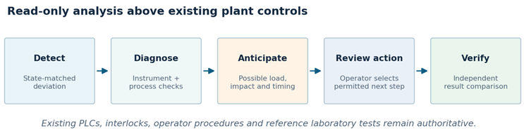
Figure 4. A neutral decision sequence for an independent, read-only intelligence layer. Neither plant controls nor laboratory verification are displaced.

In a simple pipe reach, first-order travel time equals distance divided by mean velocity. For a 1.5-mile hypothetical reach at 2 ft/s, that is 7,920 ft ÷ 2 ft/s = 3,960 seconds, or 66 minutes. Actual arrival at a municipal treatment plant may differ sharply because of pump schedules, storage, tributary flows, mixing, and changing depth. A slug also stretches and disperses; its first detectable arrival is not the same as its concentration peak.

A practical intervention budget is the remaining travel time minus measurement latency, confirmation, communications, decision time, and the lead time needed for an approved protective action. A measured anomaly 10 minutes ahead of the biology may be perfectly accurate and operationally useless. The same anomaly two hours upstream may be actionable — but only if an operator has an authorized response, sufficient storage, or diversion capability, and enough evidence to justify using it.

The analytical opportunity is to connect these timescales, not to issue automatic instructions to a plant. A read-only reasoning layer can align a source event with downstream transport, flag instrument quality, estimate a plausible arrival range and present the evidence behind a recommended check or protective response. For the manufacturer, the same event may point to a recoverable transition loss; for the wastewater operator, it may indicate a developing load or treatment risk. Those are distinct decisions, linked by the same physical event. Approval, interlocks, permits, and operating procedures remain with plant personnel.

A Valuable Anomaly Is A Better Decision, Not An Impressive Alert

The three tests readers can run on their own systems

Pick one documented out-of-range event. Draw its path from suspected source to the first station and to the affected asset. Align the timestamps against hydraulic reality, then write down the earliest safe intervention that could have changed the outcome. Finally, ask which single missing measurement would have made the conclusion more reliable. If the answer is “none,” more sensors may not be the investment to make.

SCADA is already good at threshold alarms. Well-designed neutralization controls are already good at maintaining pH where actuators and measurement are adequate. The value of an additional intelligence layer must appear where those tools stop: explaining why an excursion occurred across departmental systems, anticipating its physical consequence, and determining whether a different operating decision is warranted. If the proposed system merely reproduces alarms that operators already trust, there is no incremental benefit to buy.

The EPA’s event-detection research warns why raw alert counts are inadequate. In one evaluation, many unexpected water-quality changes were attributable to operational changes or sensor problems rather than contaminants.⁷ A useful evaluation therefore measures detection lead time, confirmed causes, false alerts per operator shift, maintenance burden, actionable response windows, and the resulting cost after implementation — not just statistical anomaly accuracy.

A credible test compares the new evidence chain with the plant's real baseline. Choose one frequent, costly event; measure source-to-sensor timing, false positives, sample agreement, response lead time, and confirmed root causes. Then record whether an operator-approved change reduced a verified material loss or wastewater load under comparable conditions. A product retained upstream must not also be counted as a second, independent wastewater saving without examining the billing basis. The most commercially important number is the measured improvement in the operating decision, not the dollar value of every anomaly the software can display.

A Practical Test: Did The Added Evidence Change A Decision?

The California case demonstrates how repeated process failures can become a serious public-infrastructure problem. The strongest monitoring response is not simply to detect an extreme value earlier. It is to establish what changed in the physical stream, which plant event could explain it, whether the instrument is trustworthy, and what approved intervention would actually stop the recurrence.

This is the architecture AquaMesh is developing: AquaLink connects to existing plant records, AquaSpectra supplies selected UV/visible measurements where an additional physical observation is justified, and process-aware software links anomalies to possible causes, consequences, and operator-reviewed actions before testing the outcome. It is intended to operate as an independent, initially read-only layer above installed controls — not as another PLC or a replacement for laboratory compliance tests. Its value would have to be demonstrated through lower confirmed losses, earlier actionable diagnosis, or reduced operator investigation effort against the plant’s current approach.

Sources and technical notes:

1. U.S. EPA, “Irwindale wire manufacturer pleads guilty to criminal wastewater discharge,” Nov. 10, 2010. https://www.epa.gov/archive/epapages/newsroom_archive/newsreleases/4333810b2f5010ee85
   2577d700686cdf.html
2. B. Balannec et al., “Treatment of dairy process waters by membrane operations for water reuse and milk constituents concentration,” Desalination 147 (2002), 89–94. https://doi.org/10.1016/S0011-9164(02)00581-7
3. Food Engineering, “How Dairy Farmers of America goes green,” Nov. 14, 2018; plant design capacity reported as four million pounds/day. https://www.foodengineeringmag.com/articles/97883-food-engineerings-2018-sustainable-plant-of-the-year-how-dairy-farmers-of-america-goes-green
4. USDA Economic Research Service, Dairy Market Outlook, updated Oct. 19, 2026; forecast 2026 all-milk price $19.90/cwt. https://www-tx.ers.usda.gov/topics/animal-products/dairy/market-outlook
5. City of San Diego, Sewer Billing Rates, Jan. 1, 2026 industrial/commercial rates. https://www.sandiego.gov/public-utilities/customer-support/sewer-billing-rates
6. M. Lepot et al., “Calibration of UV/Vis spectrophotometers,” Water Research 101 (2016), 519–534. https://doi.org/10.1016/j.watres.2016.05.070
7. U.S. EPA, Water Quality Event Detection System Challenge: Methodology and Findings, EPA/600/R-13/002. https://nepis.epa.gov/Exe/ZyPURL.cgi?Dockey=P100KLCF.txt

Alex Towfigh is founder and CEO of AquaMesh, developing AquaSpectra optical sensing and independent process-intelligence software for industrial water operations.