
How To Evaluate The Metrological Quality Of A Water Meter
By Ceferino Rodríguez Díaz

By calculating a meter’s accuracy, water providers can save money over the life of the product — and purchase the right product in the first place.
It is often difficult to determine the quality of any object with the naked eye. Sometimes we realize that something failed much sooner than we expected, and we feel frustrated about losing money or for not having been able to estimate its true quality prior to the purchase. The fault for this loss is not typically attributable to whoever manufactured the object; rather, it is due to the lack of criteria that allow us to anticipate what the performance of the object could have been and whether that performance is what we need.
This is what usually happens with water meters, where damage to the meters manifests itself in the premature loss of measurement accuracy. Until now, there has been no technical and objective criterion that allows us to evaluate or choose between several proposed meters that could be best in terms of their metrological performance. For this reason, we pose the problem below, and offer a solution, so those responsible for water treatment plants can use it in their evaluation of meters.
Problem Statement
The problem has the following factors:
- In acquisitions, we are not deciding which is the best meter among all those whose error curves are within the tunnel of admissible errors. They just have to “be in” to be considered eligible. In this case, the award is given to the cheapest meter.
- Also, the tests carried out in the laboratory only seek to determine that the meters satisfy the total scope of the measurement field within a range of admissible errors.
- When deciding on buying a water meter, we are not evaluating how long the permanence of the error curve of a meter is within the tunnel of admissible errors in terms of the volume of water that the meter could not register when its curve reaches the limits of the tunnel. This unmeasured water has a cost that must be evaluated.
Proposal For A Solution
As a first approach to solving the problem, the very low probability of intentional water consumption at flow rates Q1, Q2, and Q4 must be considered, given that these are the extreme flows of the lower and upper measurement fields. The flow rate Q1 is the minimum flow rate of the lower measurement field. The flow rate Q2 is the minimum flow rate of the upper measurement field and is, at the same time, the transition flow between the lower and upper measurement fields that are distinguished by the magnitude of their allowable errors (±5% for the lower field and ±2% for the upper field). The Q4 flow rate is the maximum flow rate of the total measurement field for which the meter can operate for a very short time, with a high probability of damage in cases of longer operating times at this flow rate.
The very low probability of intentional consumption at flow rates Q1, Q2, and Q4 excludes the possible individual use of the errors obtained (even if they are average values of a batch of meters) at these flows during meter calibration. This leads us to consider that the possible solution to the problem is found in the calculation of the integral of the meter error curve — that is, in the calculation of the area under this curve.
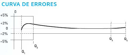
*Curva de errores=Error Curve
The error curve generally extends from Q1 to Q4, covering possible errors that may occur throughout the meter’s measurement field. In the event that, during the calibration of batches of meters on a test bench, the pressure of the bench is not sufficient to achieve the Q4 flow rate, the error curve will then extend from Q1 to the Q3 flow rate, thus covering all the possible errors up to flow rate Q3. It is then a matter of calculating the area under the curve from Q1 to Q4. If this last flow rate cannot be achieved, then the calculation of the area will be done from Q1 to Q3, in order to use this value as one of the inputs to estimate the metrological quality of a meter.
It had already been anticipated that the calculation of this area is not sufficient to determine the metrological status of the meter, so it will be necessary to calculate an ideal area that serves as a reference to compare the areas obtained from the different error curves against it.
An ideally accurate meter will have an error of 0% over its entire measurement range, from Q1 to Q4 (or from Q1 to Q3).
With the calculation of this ideal area, the overall error of a meter can now be calculated as follows:
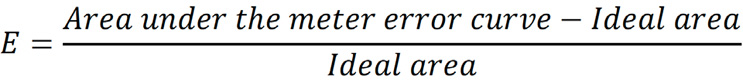
This error E represents how much the meter error curve is missing in terms of area to reach the proposed ideal area. Given the variability of the magnitude of the area under the error curve of the meter with use (entropy and wear) and knowing that the area under the error curve of a meter represents the best measurement that the meter can achieve for a given instant, then this error will characterize the metrological behavior of the meter for that same instant, so we will call it Characteristic Error Ec. The area under the error curve of the meter will be referred to hereafter as “Measured area.” (NOTE: commas [,] = decimal points [.])
Therefore:

The Measured area then comprises the following points on the error curve of the Indication Error vs. Test Flow diagram (Q1, EQ1), (Q2, EQ2), (Q3, EQ3), (Q4, EQ4), where EQ1, EQ2, EQ3, and EQ4 represent the indication errors obtained at the test flow rates Q1, Q2, Q3 and Q4.
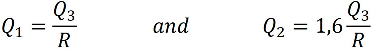
It is known that the Ratio R represents the relationship that exists between the flow rate Q3 and the flow rate Q1, like this:
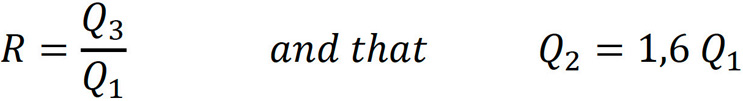
Therefore:
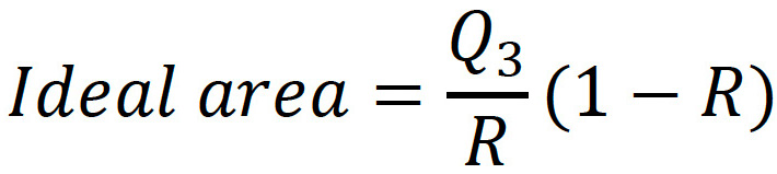
For tests up to flow rate Q3, the Ideal Area will be given by:
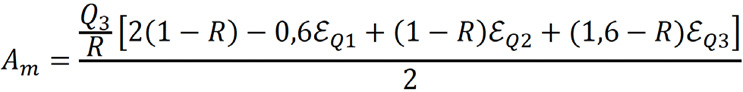
With the points mentioned above that correspond to the error curve and using these equivalences, we calculate the area under the curve for a meter (Measured Area Am), which turns out to be:
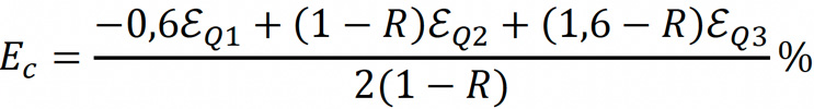
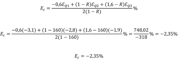
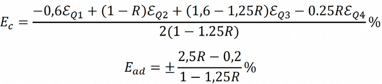
Therefore, for this case (with tests up to Q3), the Characteristic Error is:
Thus, the Characteristic Error is expressed only in terms of the errors obtained in the calibration test and in the Ratio R of the metrological class of the meter being tested. In the same way, an admissible error must be calculated. This will be determined by the area under the curve of the lines that limit the error tunnel (upper admissible limit and lower admissible limit), whose results will be related to the same Ideal Area.
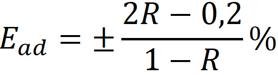
The general formula for the admissible error Ead expressed as a function of the metrological class of the meter for testing up to flow rate Q3 is:
Calculating the same developments for the tests up to flow rate Q4 results in:

The admissible error represents the operating limit of a meter, because beyond the admissible error is the zone of inadmissible errors. Therefore, the admissible error will be the limit of the useful life of a meter.
Study Cases
a) About useful life:
Suppose you want to know if the useful life of a meter (with diameter DN15 Ratio R=160 whose calibration errors are EQ1=-3,1%, EQ2=-2,8%, and EQ3=-1,9%) has ended.
Solution:
Since errors are only reported up to flow rate Q3, we calculate:
This value now is compared with the admissible error for this metrological class and tests up to Q3:
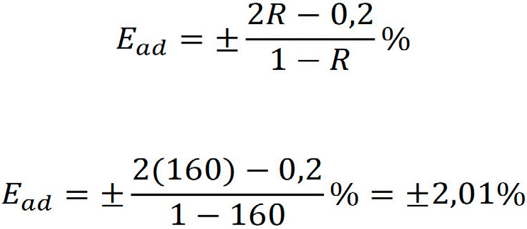
It is observed that the Ec > Ead so it can be stated that this meter exceeded the limit of its useful life.
b) Determination of metrological quality for a bid award:
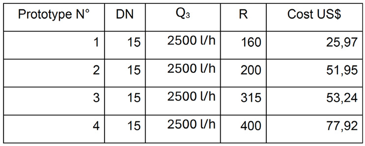
A water service provider requests proposals for the supply of meters with the following characteristics: DN15 with Q3 =2500 l/h and R≥160 in horizontal position.
The following offers were received:
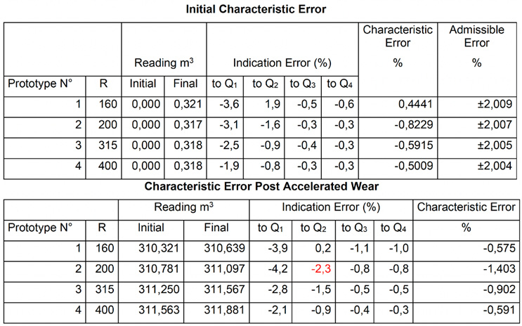
The prototypes were tested, and the following table of data was obtained that resulted from the initial calibration and a subsequent calibration performed after the 100-hour accelerated-wear test at flow rate Q4.
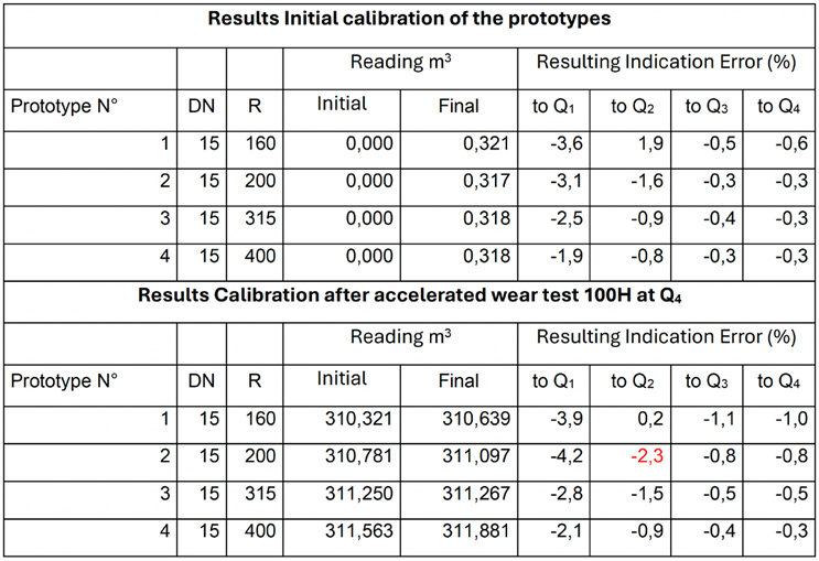
The error curves of the four prototypes in the initial calibration comply metrologically because they are all within the tunnel of admissible errors. It is also observed that after the accelerated wear to which the prototypes were subjected, the error curves of three of the meters are still completely within the tunnel of admissible errors. Prototype No. 2 presents a not very significant deviation in the indication error obtained at flow rate Q2. According to these results, the bid should be awarded to the proponent of Prototype No. 1 because it is the one with the lowest proposed cost.
Next, the application of the proposed solution is presented to verify if Prototype No. 1 is indeed the best metrological option for the award. As a first measure, the characteristic errors of the initial and post-wear test are calculated, as well as the admissible errors corresponding to the metrological classes or R Ratios involved. The formulas that apply are:
The results are presented in the following tables:
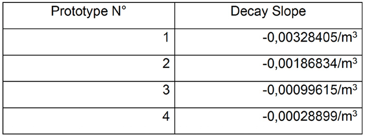
The slope of the accuracy decay curve of each prototype is calculated based on the characteristic errors found and the corresponding readings by applying the formula:

The results of the slopes of the prototypes are shown in the following table:
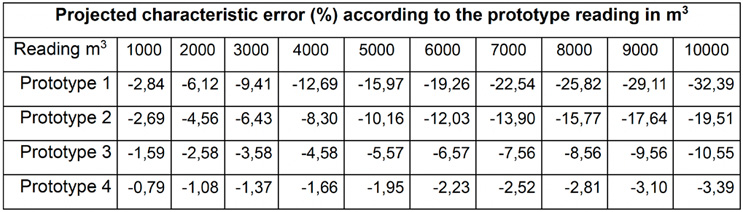
With this slope, the characteristic error can be projected for the same reading in each of the prototypes like this:

The results for different readings for each prototype are shown in the following table:
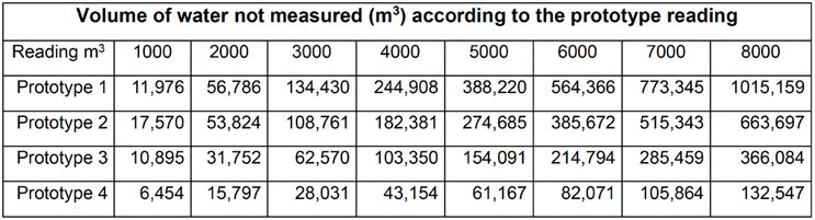
The water that each prototype will have stopped measuring (lost volume) for every 1000 m3 accumulated reading is:
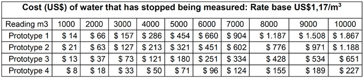
If a rate of $1,17/m3 is assumed for the reference socioeconomic stratum (4), the cost of lost water will be calculated for each prototype according to the accumulated reading. The results can be seen in the following table:
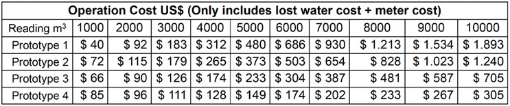
If the cost of the meter is added to this cost, the meter’s combined operation cost is obtained (for simplicity, other collateral costs are not included):
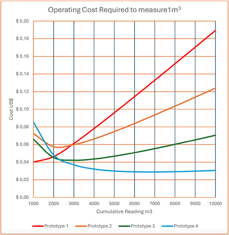
Consequently, the operating cost to measure one cubic meter within each of the previous reading ranges is obtained by dividing the total operating cost by each of the limit values of their corresponding reading ranges. The resulting operating costs are presented in the following table:
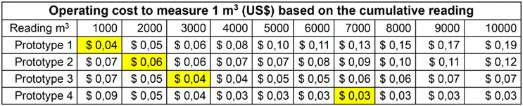
In the previous table, it can be seen that the lowest value for Prototype 1 is in the range of 1000 m3, presenting successive increments as the accumulated reading increases. For Prototype 2, the lowest value is in the range of 2000 m3; for Prototype 3, the lowest value is in the range of 3000 m3; Prototype 4 shows that the operating cost required to measure 1 m3 has its maximum value in the range of 1000 m3 range, which decreases successively until reaching a lowest value, which occurs in the range of 7000 m3. Note that for Prototype 4, from 4000 m3 to 10000 m3, the lowest measurement values of all the prototypes considered are presented. The corresponding curves are shown in the following figure.
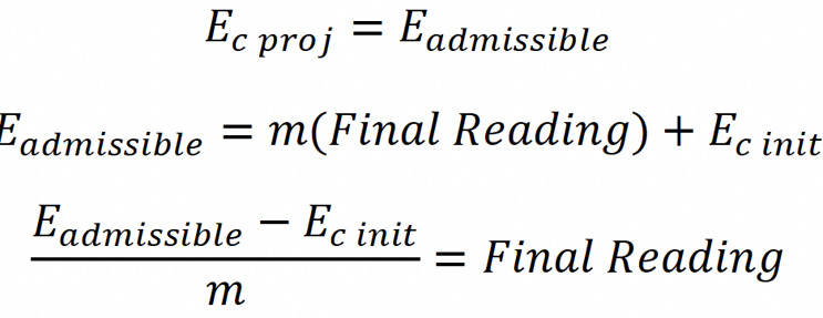
Finally, we proceed to estimate the reading that each prototype will have when its characteristic error reaches the value of the admissible characteristic error. To do this, we use the following formula:
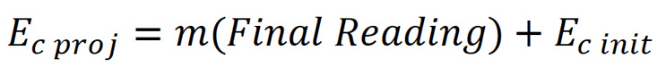
Where the projected characteristic error will be equal to the value of the admissible characteristic error for each metrological class.
For Prototype 1:
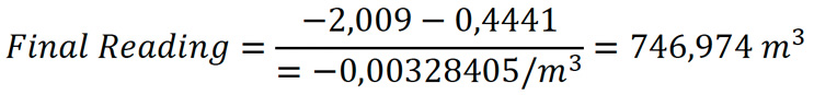
The results are presented in the following table:
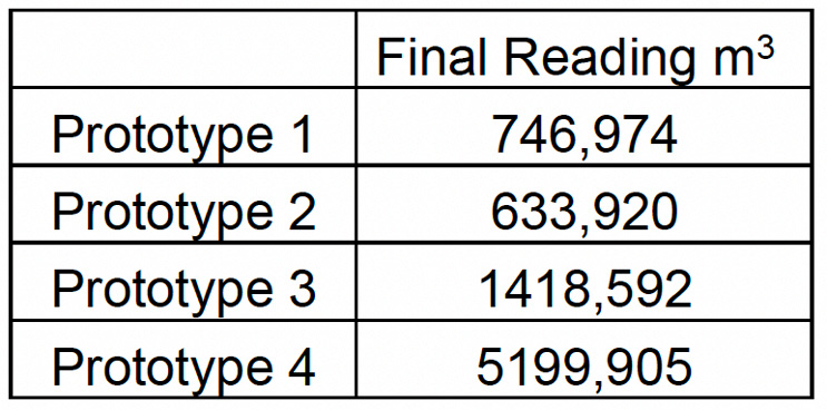
It is observed that from 747 m3 of registration, Prototype 1 begins to measure water with unacceptable errors, while for Prototype 4, its useful life extends to 5200 m3. In conclusion, Prototype 1, which seemed to be the best meter to award the purchase given its low initial cost, turns out to be an unacceptable option due to its short useful life, the large water losses that affect indicators such as the loss rate per billed user and non-revenue water losses, and the money that is lost in increasing amounts.
References:
- Bogotá Aqueduct and Sewer Company, EAAB (1989). Study of non-billed water control – Loss due to micrometering and preventive maintenance program. CNEC – Tecnoconsulta, Bogotá.
- Rodríguez, C (2016). Changing water meters due to the end of their useful life. Andesco Magazine N° 31 (p 30 -65) October 2016, Bogotá.
- Rodríguez, C (2017). Predicting the useful life of water meters from their calibration errors. Unpublished master thesis. Universidad Centro Panamericano de Estudios Superiores, México November 2017.
About The Author
 Ceferino Rodríguez Díaz, MSc., served more than 25 years as director of the aqueduct and sewer service for Empresa de Acueducto de Bogotá. His various management positions also included director of the technification and automation unit, director of non-revenue water, director of connections and meters, and director of technical services. He holds degrees from Universidad Nacional de Colombia and Universidad Centro Panamericano de Estudios Superiores (UNICEPES).